First steps in linear algebra for Quantum Computing explained (Expert resources)

Introduction

Understanding quantum computing can be daunting due to its reliance on complex mathematical concepts, particularly linear algebra. Many learners struggle with grasping these foundational principles, which hinders their ability to comprehend how quantum computing works. This challenge can be frustrating and discouraging, especially for those without access to advanced educational resources.

To address this issue, this first blog serves as a refresher on linear algebra, breaking down essential concepts such as vectors, vector notations, and vector operations. It also delves into matrix operations, including creation, addition, multiplication, transposition, and the use of Python for practical applications. By mastering these linear algebra concepts, readers will be better equipped to understand the mathematical underpinnings of quantum computing, making the learning process more accessible and less intimidating.

1. Vectors

According to Stone (2023), the space of quantum particles has four dimensions, and the particles have no size or form. Because this is difficult for us as humans to understand, we have to use math to comprehend what is going on. Many of these concepts do not reflect how things really work but describe them in a way that is understandable for us. We only observe three dimensions; the fourth dimension has no meaning to us and seems to overlap with one of the other dimensions. The three-dimensional space can be graphically shown as the Bloch Sphere, named after Felix Bloch (Stone, 2023).

Bloch Sphere rendered by Qiskit 

According to Srinivasan (n.d.), linear algebra is a branch of mathematics that deals with linear equations, linear maps, and their representations in vector spaces and matrices. Linear equations involve variables in the first order and are represented as (a1x1 + a2x2 +...+ anxn + b = 0). Vector spaces are sets of vectors that can be added together and scaled, forming n-dimensional spaces. Scalars, which have magnitude but no direction, are used to scale vectors.  Scalars are used to scale vectors. A scalar can be an imaginary number. 

Real numbers can be represented on a number line, while imaginary numbers are used to express values that cannot exist in the real world, such as the square root of -1, represented by the imaginary unit (i). Complex numbers are written as (a + bi), where (a) is the real part and (b) is the imaginary part (Stone, 2023). Complex numbers are used in Quantum Compute for qubit interference and entanglement (Microsoft, n.d.)

A Matrix is a data structure with numbers, symbols, or expressions arranged in rows and columns and they are used in various operations, including matrix multiplication. Linear maps are functions that map vectors from one vector space to another while preserving vector addition and scalar multiplication (Srinivasan, n.d.).

three dimensional vector space 

The x, y, and z axes are different from the Bloch Sphere, but this doesn't matter in three-dimensional space because the sphere or the vector map can rotate in any direction. This is not the case in two-dimensional space, where the x-axis is horizontal and the y-axis is vertical. The arrow in the sphere is a vector, which has a magnitude (length) and a direction (upwards).

1.1 Vector notations

When noting a vector, we need to write two types of information: the scale and the direction. This can be noted as (vector = ax + by + cz ), where ( x, y, ) and ( z ) are the axes, and ( a, b, ) and ( c ) are the scalar coefficients. An example could be (-6x + 2y + 1z), where the vector is located at (-6) on the x-axis, (2) on the y-axis, and (1) on the z-axis. Because ( x, y, ) and ( z ) are always in the same vector space, they are redundant (Srinivasan, n.d.). Noting a vector as ({vector} = a + b + c ) holds the same information. Noting a vector in tuple notation is ( vector = [a, b, c] ) or (vector = (a, b, c)), and in matrix notation as (vector = a b c ) as one row and three columns (Srinivasan, n.d.). When a coefficient is (0), it is not noted in the tuple notation but is noted in the matrix notation (Srinivasan, n.d.). The vector notation can in several forms, in this blog, I use bold for the vector, which is common in print (Stone, 2023).

1.2 Vector Operations

Additions of vectors are done by adding up the coefficients. Example: (v1 = (7x + 2y + 3z)) and (v2 = (x - 5y + 4z)). We can't change magnitude or direction, so we add 7 + 1, because 0x is the same as 1x or just 1. Then we subtract 2 - 5 and 3 + 4. The result is (v3 = 8x -3y + 7z) (Srinivasan, n.d.).

Calculating the magnitude (the length of the vector) of a vector with two dimensions (x,y) is: ||m|| = sqrt(x^2 + y^2) (Stone, 2023) In this case (x) is 7 and (y) is 2, so sqrt(7^2+2^2) = sqrt(49+4=53). The square root of 53 is approximately 7,28, which is the magnitude of this vector. When a vector has three dimensions, susch as v1, you need to calculate ||m|| = sqrt(x^2 + y^2 + z^2), which is sqrt(49+4+9=62) and ||m|| is approximately 7,87, so the magnitude of v1 is approximately 7,87.

Scalar multiplication scales the magnitude of a vector up and down by a scale.
Example: The scalar is 5 and multiplies v1 (7, 2,3) by 5, which is 5v1. 5v1 is calculated by (5v1 = (5*7, 5*2, 5*3), or (5v1 = (35,10,15)). The vector has now a magnitude of times 5 and the direction remains the same (Srinivasan, n.d.).

Vector transposing turns a row vector into a column vector and vice versa. This is done to multiply vectors. Example: The picture below shows vector transposing. v1 (row vector) is transposed to v1.T (column vector) (Stone, 2023). The T should be in superscript, but because of restrictions of this blog platform, I used the .T notation.

Vector transposing is necessary when you multiply vectors manually. It is not necessary when a scripting tool like Python is used, which is described later on in this blog.

The dot product, or inner product is calculated by multiplying two vectors and adding up the numbers. The dot product is not a vector, but one scalar. 

Example: (v1 = (7 + 2y + 3z)) and (v2 = (x - 5y + 4z)). The calculation is (7*1 + 2*-5 + 3*4), which is (7-10+12) and the dot product, or inner product, is 9 (Srinivasan, n.d.).

The cross product is the multiplication of two vectors and results in a new vector. This is only possible when in the matrix notation and the first matrix has the same number of columns as the second matrix has number of rows. In case the second vector has more or less rows than the first vector has columns, you can't calculate the cross product (Srinivasan, n.d.).
Example by Srinivasan (n.d.):

First we multiply 2 by 4 and 3 by -5, which is (2*4=8) and (3*-5 = -15). Then we subtract both numbers, which is (8--15), or (8+15 = 23). Then (7*4 - 3*1 = 25) and (7*-5 - 2*1 = -35 - 2 = -37).
The cross product = (23, 25,-37). 

An orthogonal basis is a set of vectors that can be combined to represent any other vector in the vector space. These vectors are perpendicular to each other and, when normalized, have a length of one, forming an orthonormal basis (Stone, 2023). In quantum computing, the vectors ((1,0)) and ((0,1)) are important because they represent the base states for qubits, often denoted as (|0>) and (|1>).  Any vector in the space can be represented as a linear combination of these orthogonal basis vectors (Stone 2023).
Example:  the vector (7,2) can be expressed as (7 * (1,0) + 2 * (0,1) = (7,2)).

2 Matrix Operations with Python

Linear algebra is best used with matrices and is supported by python very well.
A matrix can hold all kinds of information and there is no limit to how many items it can hold. A matrix has rows and columns, but could also be just one row (a row matrix) or one column (column matrix). Matrices can be added and multiplied using the same methodology as just described. A matrix with 3 rows and 5 columns is called a 3 by 5 matrix (Srinivasan, n.d.).

For this course, I used Jupyter Lab (https://jupyter.org/try-jupyter/lab/) to work with Python, because it's straight forward and nothing has to be installed.

2.1 Creating a new matrix

Creating a matrix with python can be done in various ways. Some are shown below in examples by Srinivasan (n.d.):

Matrix a is created by stating numbers in one row and then reshape to a column with 3 rows and 3 columns.

Matrix b is created by using a loop, with numbers in the range starting with 0 and ending before 18, with an interval of two. In this case, you need to make sure that the numbers you receive fit in the matrix as stated. In case you generate 18 numbers (interval 1), it won't fit in a 3x3 matrix.

Matrix c is created with a loop, with numbers up to 6.

Matrix d is created by stating numbers in rows. In this way, you can add in the numbers you want and in the format you want. In this case, 2 rows and 2 columns.

2.2 Matrix addition

It is easy to add two matrices and create the results in a third. Below is show how matrix (a) is added to matrix (b) and the results.

Subtracting is about the same as shown below

2.3 Matrix Multiplication

Multiplying matrices with python is much easier to calculate than by hand as shown earlier. However, there is a catch. The command (a*b) does work in python, but the result is wrong. The multiplication is one of an array of numbers, but does not follow the rules for multiplying matrices.

In the picture below, you can see (and calculate by hand) that the result of (a*b) does not show the correct output.

Another issue is that the command (np.dot(a,b)) does show the correct matrix as a result, but you would expect the dot product, a scalar, instead. You can use this command to multiplying matrices, but it will return a scalar when the matrix has one row. For consistency, it's better not to use this method for matrix multiplication.

The most clear and best way for matrix multiplication is the use of (np.matmul(a,b)), which is designed for matrix multiplications (Srinivasan, n.d.).

2.4 Matrix Transposal

Transposal creates a new matrix and switches the rows and columns. It's important to note that a transposed matrix is a new matrix and not the same in another format. There are two ways, one is (a.T) and the other is (np.transpose(a)) (Srinivasan, n.d.).

2.5 Diagonal matrices

Diagonals are important in linear algebra and the first important number is the trace. The trace is the sum of the numbers in the diagonal from top left to bottom right (1,22,12)(Srinivasan, n.d.). Calculating the trace is only possible when the matrix has an equal number of rows and columns, however, Python will give you a wrong output. The python command for calculating the trace is shown below.

Good thing to know is when you multiply a matrix, even if it's not symmetric, with it's own transposed version, the result is always a symmetric matrix (Srinivasan, n.d.). In the picture below, you see the non-symmetric matrix (c), then the result after multiplication with its transposed version and the result of the trace (55).

A vertical matrix is a matrix with the vertical cells filled and the other cells only have zeros. A vertical matrix where the cells are filled with ones (and the other cells with zero) is called an identity matrix (Srinivasan, n.d.). 

In the picture below, matrix (g) is created and displayed. The vertical is filled with (2) and the other cells are filled with (0). Matrix (g) is a vertical matrix.
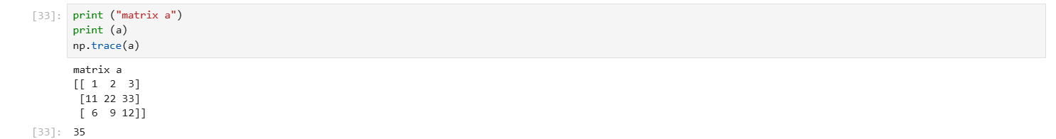
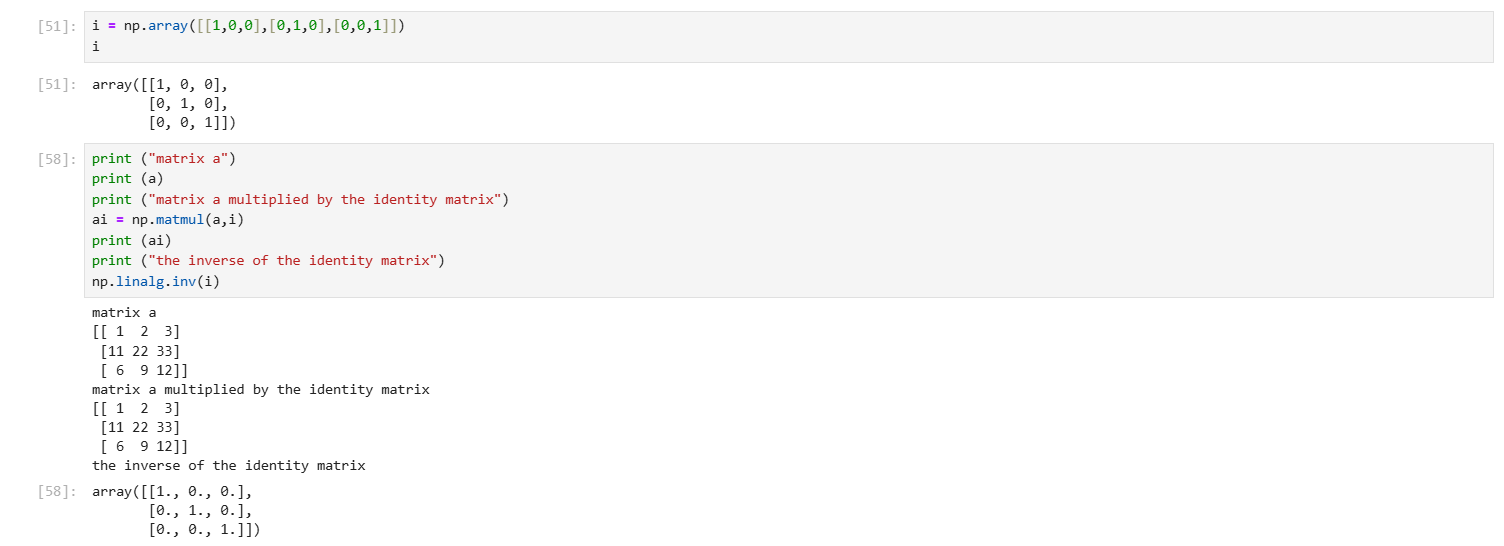
Matrix (i) is created and displayed below matrix (g). The vertical is filled with (1) and the other cells are filled with (0). Matrix (i) is an identity matrix.

The identity matrix is special, because, when a matrix is multiplied by the identity matrix, the result is always the original matrix and the inverse of the identity matrix is also an identity matrix.

The picture below shows the creation of the identity matrix, the multiplication of matrix (a) with the identity matrix (i) and the inverse of the identity matrix.

A zero matrix is a matrix filled with zeros. A zero matrix can have any size, but note that a zero matrix with a different size are unequal to each other. For example, A 2x2 zero matrix is a different matrix than an 1x2 matrix (Srinivasan, n.d.).

2.6 Inverse matrix

When a matrix multiplied by another matrix results in an identity matrix, then both matrices are inverses of each other. 

In the picture below, the creation of two matrices are shown, matrix (h) and matrix (j). The multiplication of matrix (h) by matrix (j) results in an identity matrix (Srinivasan, n.d.).

There is an easier way to find the inverse of a matrix, shown below.

In case a matrix doesn't have an inverse, you'll get an error. Not every matrix has an inverse.

2.7 Hadamard product

The last one is a multiplication of two matrices, but on element base. Earlier in this blog, I explained that matrix * matrix doesn't multiply the matrix. What it does is element based multiplication and that is the Hadamard product. A better way to do this is using multiply() as shown below.

You can see the two matrices (h and j) and the result of multiply (h,j). The result is the same as when you use (h*j). I favor multiply, because it is more clear what we are actually doing and what is the result is going to be.

3. Conclusion

In this blog, we've revisited the fundamental concepts of linear algebra, which are essential for understanding quantum computing. By exploring vectors, vector notations, and vector operations, we've laid the groundwork for visualizing the behavior of quantum particles in multi-dimensional spaces. Additionally, we've delved into matrix operations, including creation, addition, multiplication, transposition, and the practical use of Python to perform these operations.

Mastering these linear algebra concepts is crucial for anyone looking to comprehend the mathematical underpinnings of quantum computing. With this solid foundation, you'll be better prepared to tackle more advanced topics in quantum computing and apply these principles to real-world scenarios. As you continue your journey, remember that understanding these basics will make the complex world of quantum computing more accessible and less intimidating.

Sources

Microsoft (n.d.). https://quantum.microsoft.com/en-us/insights/education/concepts/quantum-math#:~:text=The%20use%20of%20complex%20numbers,key%20features%20of%20quantum%20mechanics.

Srinivasan (n.d.). https://www.percipio.com/courses/23da95d4-b1e2-46c7-a189-c9437f33de5c/videos/88dddff0-134b-4237-879c-1e59b7b4c495

Stone, O. C. (2023, 17 april). Learn quantum computing - Quantum Computing Fundamentals [Video]. LinkedIn. https://www.linkedin.com/learning/quantum-computing-fundamentals/learn-quantum-computing?contextUrn=urn%3Ali%3AlearningCollection%3A7013770329806249984&u=46118444